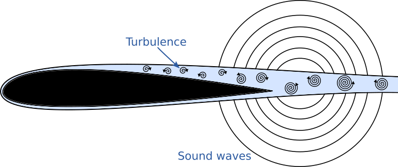
Machine learning of airfoil self-noise with interpretable polynomial trees

The NASA data set comprises different size NACA 0012 airfoils at various wind tunnel speeds and angles of attack.

UCI Machine Learning repository

Feature	Description	Units
\(f\)	Frequency	Hz
\(\alpha\)	Angle of attack	Degrees
\(U_{\infty}\)	Free-stream velocity	m
\(C\)	Airfoil chord length	m/s
\(\delta^*\)	Suction side boundary layer thickness	m

Output is SPL, the scaled sound pressure level, in decibels.

import numpy as np
import equadratures as eq
import pandas as pd
import matplotlib.pyplot as plt

random_state = 4
data = pd.read_csv('https://archive.ics.uci.edu/ml/machine-learning-databases/00291/airfoil_self_noise.dat',delimiter='\t',
                  names=['Frequency','AoA','Chord','Velocity','Thickness','spl'])
y = data.spl.to_numpy()
X = data.drop('spl',axis = 1).to_numpy()
X_train, X_test, y_train, y_test = eq.datasets.train_test_split(X, y, train=0.75, \
                                                                random_seed=random_state)

# Define a helper scorer/plotting function
def test_model(model):
    ypred_train = model.predict(X_train)
    ypred_test  = model.predict(X_test)

    fig, ax = plt.subplots()
    ax.plot(y_train,ypred_train,'o',alpha=0.6,mec='k',label='train')
    ax.plot(y_test,ypred_test,'o',alpha=0.6,mec='k',label='test')
    ax.plot([np.min(y_test),np.max(y_test)],[np.min(y_test),np.max(y_test)],
            'k--',zorder=10,lw=2)
    ax.set_aspect(1)
    ax.set_xlabel('Actual')
    ax.set_ylabel('Predicted')
    ax.set_xlim([np.min(y_test),np.max(y_test)])
    ax.set_ylim([np.min(y_test),np.max(y_test)])
    ax.grid('on')
    ax.legend()
    plt.show()

    print('Training MAE = %.2f' %(eq.datasets.score(y_train,ypred_train,'mae')))
    print('Test MAE = %.2f' %(eq.datasets.score(y_test,ypred_test,'mae')))

from sklearn.tree import DecisionTreeRegressor
DT = DecisionTreeRegressor(criterion='mse',max_depth=10,
                           min_samples_leaf=2,random_state=random_state)
DT.fit(X_train,y_train)
test_model(DT)

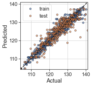
Training MAE = 1.10
Test MAE = 2.23

from sklearn.ensemble import RandomForestRegressor
# Random forest with fully grown trees
RF = RandomForestRegressor(n_estimators=100,criterion='mse',max_depth=None,
                           random_state=random_state)
RF.fit(X_train,y_train)
test_model(RF)

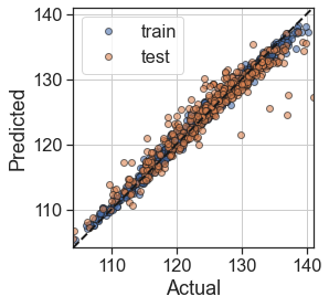
Training MAE = 0.50
Test MAE = 1.42

order = 3        #or deeper tree with order=1
max_depth = 3

tree = eq.PolyTree(splitting_criterion='loss_gradient', max_depth=max_depth,
                    order=order, poly_method='elastic-net',
             poly_solver_args={'max_iter':20,'verbose':False,'alpha':1.0,'nlambdas':20,
                         'crit':'CV'})

tree.fit(X_train,y_train)

test_model(tree)

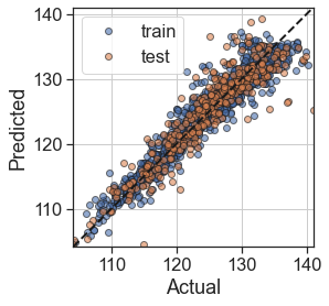
Training MAE = 1.49
Test MAE = 1.94

References

[1]: Brooks, T. F., Pope, D. S., and Marcolini A. M. (1989), Airfoil self-noise and prediction. Technical report, NASA RP-1218.