In [1]:
import IPython.core.display as di # Example: di.display_html('<h3>%s:</h3>' % str, raw=True)
di.display_html('<script>jQuery(function() {if (jQuery("body.notebook_app").length == 0) { jQuery(".input_area").toggle(); jQuery(".prompt").toggle();}});</script>', raw=True)
In [2]:
import matplotlib.pyplot as plt;
# %matplotlib notebook
Basis
A multi-index is a set of indices that enumerates composite univariate polynomial orders that are involved in forming the multivariate basis. As we intend to approximate \(f\) via a finite number of polynomials \(\boldsymbol{\phi_i}\), we restrict indices \(\boldsymbol{i}\) to lie in a finite multi-index set \(\mathcal{I}\). Whilst considerable flexibility in specifying these multi-index sets exists, well-known \(\mathcal{I}\) include tensor product index sets, total order index sets, Euclidean degree spaces [1] , and hyperbolic spaces [2] . Each of these index sets in \(d\) dimensions is well-defined given a fixed \(k \in \mathbb{N}_0\), which indicates the maximum polynomial degree associated to these sets. Tensor product index sets are characterised by \begin{equation} \max_k i_k \leq k, {\tag{1}} \end{equation} and have a cardinality (number of elements) equal to \((k+1)^d\). Total order index sets contain multi-indices satisfying \begin{equation} \sum_{j=1}^d i_{j} \leq k {\tag{2}} \end{equation} They effectively disregard some higher order interactions between dimensions present in tensorised spaces, and a total order index set \(\mathcal{I}\) has cardinality \begin{equation} \left| \mathcal{I} \right|=\left(\begin{array}{c} k+d\\ k \end{array}\right). {\tag{3}} \end{equation} For a hyperbolic space index set, \begin{equation} \left(\sum_{j=1}^{d}i_{j}^{q}\right)^{1/q} \leq k, \label{eq:hyperbolic-space}{\tag{4}} \end{equation} where \(q\) is a user-defined constant that can be varied from 0.2 to 1.0. When this parameter is set to unity \(q=1\), the hyperbolic index space is equivalent to a total order index space. For values less than unity higher-order interactions terms are eliminated as discussed before [2].
For illustrative purposes, plots of the main multi-index sets associated with \(d=2\) and with a maximum univariate degree of 14 are shown below.
In [3]:
imgs = [
    'Figures/tensor.png',
    'Figures/total.png',
    'Figures/hyperbolic.png'
]

nimgs = len(imgs)
In [4]:
def grid_display(list_of_images, list_of_titles=[], no_of_columns=2, figsize=(10,10)):

    fig = plt.figure(figsize=figsize)
    column = 0
    for i in range(len(list_of_images)):
        column += 1
        #  check for end of column and create a new figure
        if column == no_of_columns+1:
            fig = plt.figure(figsize=figsize)
            column = 1
        fig.add_subplot(1, no_of_columns, column)
        plt.imshow(list_of_images[i])
        plt.axis('off')
        if len(list_of_titles) >= len(list_of_images):
            plt.title(list_of_titles[i], fontdict={'fontsize': '30'})

images = [plt.imread(image) for image in imgs]
grid_display(images, ['(a)', '(b)', '(c)'], 3, (30,30))
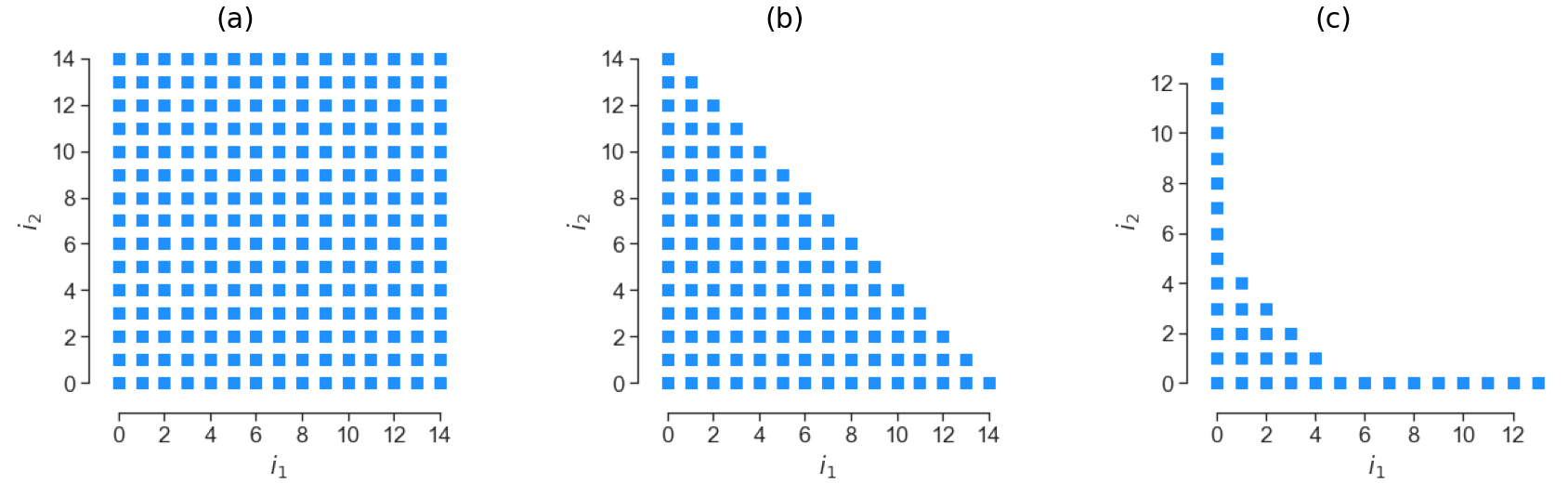
Figure 1: Multi-indices for \(d=2\) with a maximum univariate degree of 14 for: (a) tensor order; (b) total order; (c) hyperbolic space.
Of particular importance is the growth and interaction of the higher order terms. In total order and hyperbolic spaces, higher order interaction terms are significantly reduced. For many physical systems, these type of sparser basis have found utility as lower order interactions are often far more dominant. Another important consideration when choosing a multi-index is the level of anisotropy along each dimension. For instance, one can have different maximum degrees in each direction.