Foundations II: Orthogonal polynomials#
In this tutorial we describe how one can construct orthogonal polynomials in Effective Quadratures. These polynomials have the property of being orthogonal to each other under integration with respect to a specific probability measure. That is, they obey the following:
In this first part, let’s consider univariate orthogonal polynomials—it turns out that multivariate orthogonal polynomials can be constructed as products of univariate ones. For starters, we consider Legendre polynomials—orthogonal with respect to the uniform weight function. We define a Parameter \(s\) with \(\rho(s) \sim \mathcal{U}[-1,1]\).
In [2]:
import numpy as np
import matplotlib.pyplot as plt
import equadratures as eq

order = 5
s1 = eq.Parameter(lower=-1, upper=1, order=order, distribution='Uniform')
Setting order=5 implies that we restrict our attention to the first five orthogonal polynomials. The polynomials can be evaluated on a grid of \(N\) points \((\lambda_{j})_{j=1}^N\), forming the Vandermonde-type matrix \(\mathbf{P}\) where
Here, \(p\) denotes the maximum polynomial order, 5 in our case. The matrix for 100 evaluations within \([-1,1]\) can be generated as below:
In [3]:
myBasis = eq.Basis('univariate')
myPoly = eq.Poly(s1, myBasis, method='numerical-integration')
xo = np.linspace(-1., 1., 100)
P = myPoly.get_poly(xo)
Using this matrix, we can generate plots of the polynomials shown below (this plot can also be generated with s1.plot_orthogonal_polynomials()).
In [4]:
fig = plt.figure()
ax = fig.add_subplot(1,1,1)
plt.plot(xo, P[0,:], lw=2, label='Order 0')
plt.plot(xo, P[1,:], lw=2, label='Order 1')
plt.plot(xo, P[2,:], lw=2, label='Order 2')
plt.plot(xo, P[3,:], lw=2, label='Order 3')
plt.plot(xo, P[4,:], lw=2, label='Order 4')
plt.plot(xo, P[5,:], lw=2, label='Order 5')
plt.legend(loc='upper center', bbox_to_anchor=(0.5, 1.30), ncol=3, fancybox=True, shadow=True)
plt.xlabel('$s$', fontsize=18)
plt.ylabel('Polynomials', fontsize=18)
plt.show()
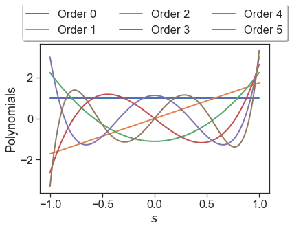
A few remarks are in order regarding this plot. Standard Legendre polynomials are orthogonal via
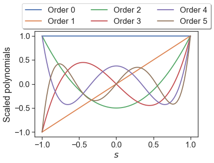
where \(\delta_{ij}\) is the Kronecker delta. In Effective Quadratures, we modify all orthogonal polynomials such that the right hand side of this expression is unity when \(i=j\). Re-introducing these scaling factors, we now can plot the standard Legendre polynomials; these are reported in the Wikipedia entry.
In [5]:
factor_0 = 1.
factor_1 = 1.0 / np.sqrt(2.0 * 1.0 + 1.)
factor_2 = 1.0 / np.sqrt(2.0 * 2.0 + 1.)
factor_3 = 1.0 / np.sqrt(2.0 * 3.0 + 1.)
factor_4 = 1.0 / np.sqrt(2.0 * 4.0 + 1.)
factor_5 = 1.0 / np.sqrt(2.0 * 5.0 + 1.)

fig = plt.figure()
ax = fig.add_subplot(1,1,1)
plt.plot(xo, factor_0 * P[0,:], lw=2, label='Order 0')
plt.plot(xo, factor_1 * P[1,:], lw=2, label='Order 1')
plt.plot(xo, factor_2 * P[2,:], lw=2, label='Order 2')
plt.plot(xo, factor_3 * P[3,:], lw=2, label='Order 3')
plt.plot(xo, factor_4 * P[4,:], lw=2, label='Order 4')
plt.plot(xo, factor_5 * P[5,:], lw=2, label='Order 5')
plt.legend(loc='upper center', bbox_to_anchor=(0.5, 1.30), ncol=3, fancybox=True, shadow=True)
plt.xlabel('$s$', fontsize=18)
plt.ylabel('Scaled polynomials', fontsize=18)
plt.show()
Quadrature Points#
There is an intimate relationship between orthogonal polynomials and quadrature points. In this section, we demonstrate how one can use Effective Quadratures to compute univariate quadrature rules. Consider the task of integrating the function
where the measure \(\rho \left( s \right)\) is the uniform distribution over \([-1,1]\). Our task is to numerically approximate this integral using a quadrature rule, i.e.,
where the pair \(\left\{ \lambda_{i} , \omega_i \right\}_{i=1}^{N}\) represents an N-point quadrature rule. The constant \(2\) arises because we are integrating over the range of \([-1,1]\) and our quadrature weights sum up to \(1\). To obtain such points in Effective Quadratures, one uses the following commands.
In [6]:
order = 4
myParameter = eq.Parameter(lower=-1, upper=1, order=order, distribution='Uniform')
myBasis = eq.Basis('univariate')
myPoly = eq.Poly(myParameter, myBasis, method='numerical-integration')
points, weights = myPoly.get_points_and_weights()
The above quadrature rule is known as Gauss-Legendre, because we used Legendre polynomials (by specifying a uniform distribution) and derived quadrature points and weights from them—All these are done behind the scenes. In practice if one wishes to evaluate an integral, the weights must be scaled depending on the domain of integration. Let \(f(x) = x^7 - 3x^6 + x^5 - 10x^4 + 4\) be our function of choice, defined over the domain \([-1,1]\). The analytical integral for this function is 22/7. Now using our 5-point Gauss-Legendre quadrature rule, we obtain
In [7]:
def function(x):
        return x[0]**7 - 3.0*x[0]**6 + x[0]**5 - 10.0*x[0]**4 +4.0

integral = float( 2  * np.dot(weights , eq.evaluate_model(points, function) ) )
integral
Out[7]:
3.142857142857177
which yields 3.14285714 and is equal to 22/7 up to machine precision. Note that the constant 2 arises because we are integrating over \([-1,1]\) with the uniform measure, which has a density of 1/2.
Now, in addition to standard Gauss-Christoffel quadrature rules for a wide range of distributions, Effective Quadratures also has Gauss-Christoffel-Lobatto rules, which feature end-points and Gauss-Christoffel-Radau rules, which are variations on the standard Gauss quadrature rules that include either or both of the end points of the integration domain. To use these rules, we can specify the endpoints option when defining the Parameter object.
In theory, these points should yield the same accuracy as before. To verify the accuracy of these points, we use the same code as above.
In [8]:
s2 = eq.Parameter(lower=-1, upper=1, order=order, distribution='uniform', endpoints='lower')
s3 = eq.Parameter(lower=-1, upper=1, order=order, distribution='uniform', endpoints='upper')
s4 = eq.Parameter(lower=-1, upper=1, order=order, distribution='uniform', endpoints='both')

myPoly2 = eq.Poly(s2, myBasis, method='numerical-integration')
myPoly3 = eq.Poly(s3, myBasis, method='numerical-integration')
myPoly4 = eq.Poly(s4, myBasis, method='numerical-integration')

points2, weights2 = myPoly2.get_points_and_weights()
points3, weights3 = myPoly2.get_points_and_weights()
points4, weights4 = myPoly2.get_points_and_weights()

integral2 = float( 2  * np.dot(weights2 , eq.evaluate_model(points2, function) ) )
integral3 = float( 2  * np.dot(weights3 , eq.evaluate_model(points3, function) ) )
integral4 = float( 2  * np.dot(weights4 , eq.evaluate_model(points4, function) ) )
integral2, integral3, integral4
Out[8]:
(3.142857142857182, 3.142857142857182, 3.142857142857182)
Again, the outputs should be equal to the analytical value up to machine precision.
Index-sets#
In practice, we are often interested in modeling functions of several variables. How can we extend orthogonal polynomials to multiple dimensions? One straightforward observation is that—assuming that all input variables \(\mathbf{s} = \{s_1,s_2,...,s_d\}\) are independent, we can decompose the joint input distribution as the product of marginals in each dimension:
This implies that multivariate polynomials of the form are orthogonal:
where each \(\psi_i\) comes from the orthogonal polynomial set for the respective dimension. Thus, to specify a multivariate orthogonal polynomial, we need a \(d\)-vector that specifies the degree of polynomial in each dimension instead of a single number as in the univariate case. This vector is known as a multi-index, and the possible set of multi-indices in a multivariate basis is known as the index set. There are five different types of index sets in Effective Quadratures:
Option |
Index set |
Parameters |
|---|---|---|
1 |
|
List of max. individual orders |
2 |
|
List of max. individual orders |
3 |
|
Growth rule and level parameter |
4 |
|
List of max. individual orders and a truncation parameter |
5 |
|
List of max. individual orders |
In what follows, we will briefly demonstrate how we construct them and visualise them in three dimensions. We begin by defining a tensor grid index set in three dimensions, and we plot the three dimensional tensorial grid using the inbuilt method plot_index_set().
In [9]:
tensor = eq.Basis('tensor-grid', [4,4,4])
tensor.plot_index_set()
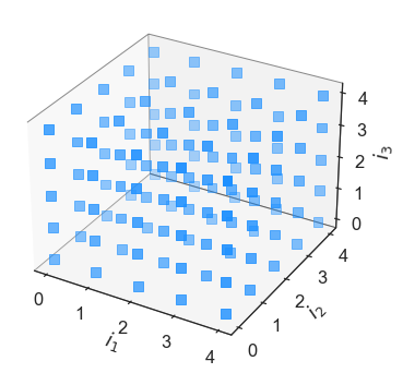
It is readily apparent that the tensor grid index set has virtually every element within the order [4,4,4] cube. Lets suppose that one does not want to afford \(4^3\) computations, necessary to approximate all the coefficients associated with a tensor index set multivariate polynomial. One can then opt for a sparse grid, which are select linear combinations of select tensor products. In Effective Quadratures, they can be declared as follows:
In [10]:
sparse = eq.Basis('sparse-grid', level=2, growth_rule='linear',orders=[4,4,4])
sparse.plot_index_set()
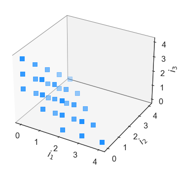
Here \(a\) is the select tensor product grid used, and \(b\) is the linear coefficients used when combining the tensor product grid. While the code can perform integrations and coefficient approximation using sparse grids, we recommend users to stick to the effective subsampling approach that uses least squares. In both theory and practice, the results are identical. We now move on to the three other index sets: Total order, Euclidean and a Hyperbolic basis.
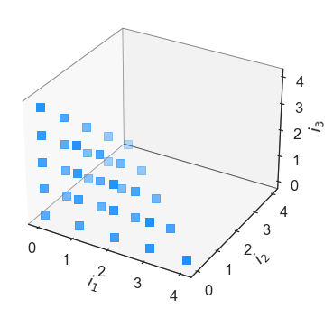
In [11]:
total = eq.Basis('total-order', [4,4,4])
total.plot_index_set()
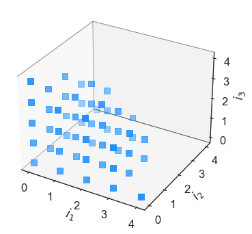
In [12]:
euclid = eq.Basis('euclidean-degree', [4,4,4])
euclid.plot_index_set()
In [13]:
hyper = eq.Basis('hyperbolic-basis', [4,4,4], q=0.5)
hyper.plot_index_set()
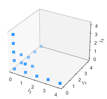
The hyperbolic basis takes in a \(q\) value, which varies between 0.1 and 1.0. Feel free to play around with this parameter and see what the effect on the total number of basis terms are. This is known as the cardinality of the index set, and can be returned with:
In [14]:
hyper.get_cardinality()
Out[14]:
16